B_HIT.st tutorial

filter process

First, let us load the packages that will be necessary for the analysis.

import B_HIT
import scanpy as sc
import anndata as ad
import matplotlib.pyplot as plt

We can download the full dataset through the github(web). Meanwhile, we use genes closely related to B cells to distinguish B cells from other cells.

adata = sc.read("./data/twosamples.h5ad")
signature = ["CD79A", "CD79B", "MS4A1", "CD79A", 'CD79B', "MZB1", "JCHAIN", "IGHA1", 'IGHG1', 'IGHG3']
score_name = 'Bcell_enrichment'
sc.tl.score_genes(adata, gene_list=signature, score_name=score_name)

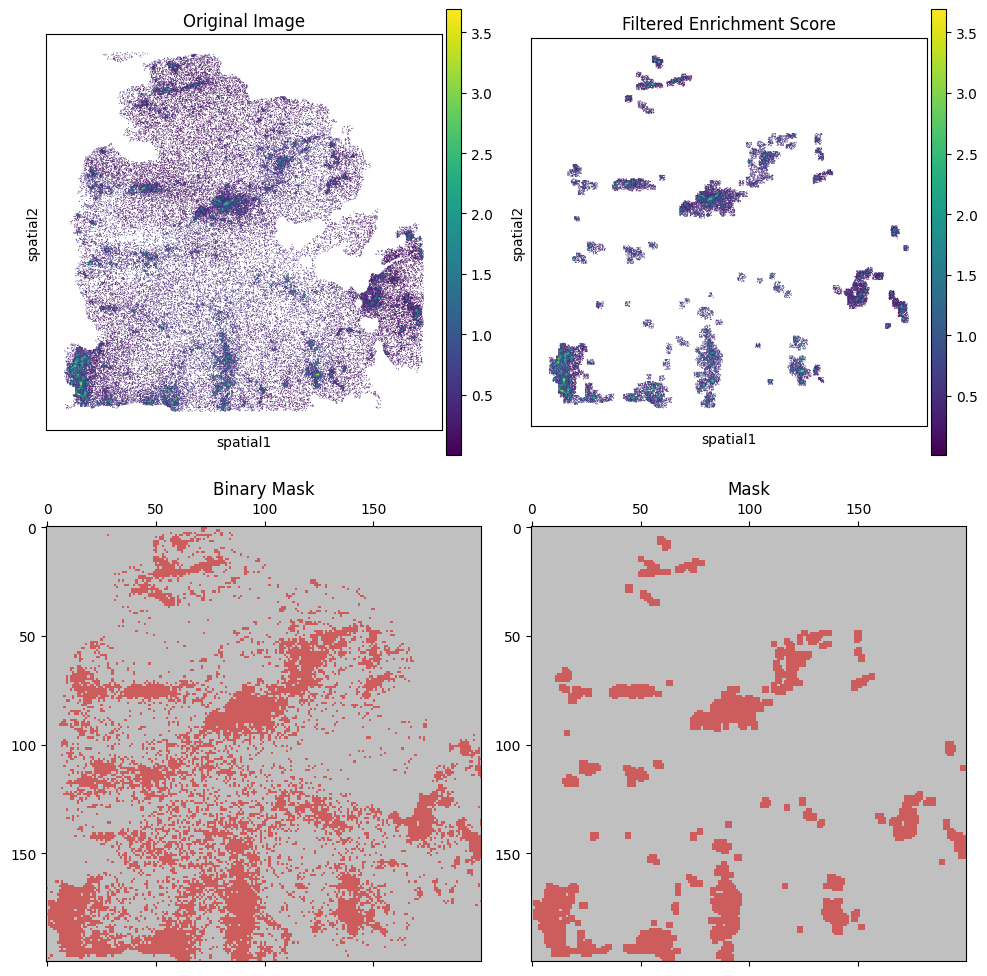
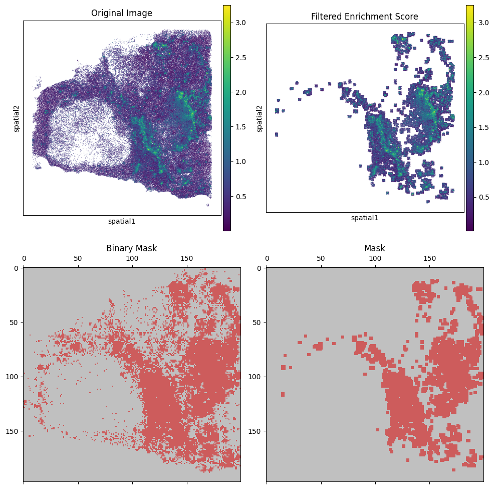
We filter the cells by B_HIT.st.tl.kde_filter, plot them by B_HIT.st.pl.enrichment_score, visualizing the results.

adata = adata[adata.obs[score_name]>0]
ad_cut = []
samples = set(adata.obs['sample'])
for sample in samples:
    print(sample)
    adata_tmp = adata[adata.obs['sample'].isin([sample])]
    ad_cut.append(B_HIT.st.tl.kde_filter(adata_tmp, score_name))
    B_HIT.st.pl.kde_results(adata_tmp, score_name, plot_masks=True, plot_enrichment=True, figsize=(10, 10), spot_size=50)
enrichedAd = ad.concat(ad_cut)
enrichedAd = adata[enrichedAd.obs.index]
print(enrichedAd)

P0608_CC
Step 1 (Prepare): 0.13 s
Step 2 (kde score): 58.16 s
Step 3 (obtain legal coords): 1.02 s
P1121_LM
Step 1 (Prepare): 0.99 s
Step 2 (kde score): 134.49 s
Step 3 (obtain legal coords): 6.29 s
View of AnnData object with n_obs × n_vars = 152726 × 25091
    obs: 'n_genes', 'n_genes_by_counts', 'total_counts', 'total_counts_mt', 'pct_counts_mt', 'annotations', 'GEX_leiden', 'celltype', 'epiHRC', 'epiEMT', 'epiStem', 'CancerClass', 'celltype_1', 'T_score', 'loc', 'loc_1', 'celltype_2', 'Ribosome-related', 'TA-like', 'InjureRepair', 'Absorptive-like', 'CryptBottom-like', 'Secretory-like', 'Tuft-like', 'cancerType', 'Others', 'MuscleCell', 'B', 'Endothelial', 'NK', 'Macrophages', 'Fibroblast', 'T', 'DC', 'Malignant', 'sample', 'macro_class', 'SPP1+IL1+ macro', 'SPP1+TREM2+ macro', 'SPP1+MMP+ macro', 'FOLR2+ macro', 'CXCL9+ macro', 'T_subtype', '_scvi_batch', '_scvi_labels', 'spatial_cluster', 'patient', 'tissue', 'spatial_cluster_1', 'spatial_cluster_2', 'TLS', 'Bcell_enrichment'
    var: 'mt'
    uns: '_cellcharter', '_scvi_manager_uuid', '_scvi_uuid', 'rank_genes_groups', 'spatial_cluster_colors', 'spatial_fov', 'spatial_neighbors'
    obsm: 'X_cellcharter', 'X_pca', 'X_scVI', 'X_umap', 'spatial'
    obsp: 'connectivities', 'distances', 'spatial_connectivities', 'spatial_distances'

cluster process

DBSCAN can be used to classify and visualize the filtered results.

res_sample_ad = [] 
samples = set(enrichedAd.obs['sample']) 

for sample in samples:
    ad_sample = enrichedAd[enrichedAd.obs['sample']==sample].copy()
    ad_sample = B_HIT.st.tl.dbscan_filter(ad_sample, eps=100, min_samples=50)
    res_sample_ad.append(ad_sample)

res_ad = ad.concat(res_sample_ad) 

Generate neighbors from the data, and use ClusterAutoK to determine the most appropriate number of clusters.

B_HIT.st.gr.aggregate_neighbors(enrichedAd, n_layers=3, 
                                use_rep='X_scVI', out_key='X_scVI_hop3',
                                sample_key='sample', connectivity_key='spatial_connectivities')
model = B_HIT.st.tl.ClusterAutoK(n_clusters=(2,6), max_runs=2)
model.fit(enrichedAd, use_rep='X_scVI_hop3')
B_HIT.st.pl.silhouette_scores(model, (2, 6))

Iteration 1/2
[[0.16185006, 0.15761554, 0.10639121, 0.09760838, 0.11401569]]
Iteration 2/2
[[0.16185006, 0.15761554, 0.10639121, 0.09760838, 0.11401569], [0.16148472, 0.15749086, 0.10639121, 0.13395573, 0.10797189]]

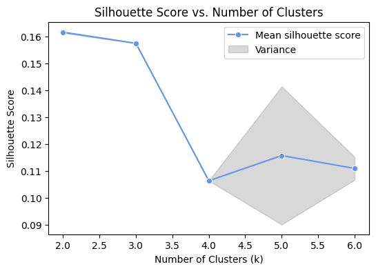
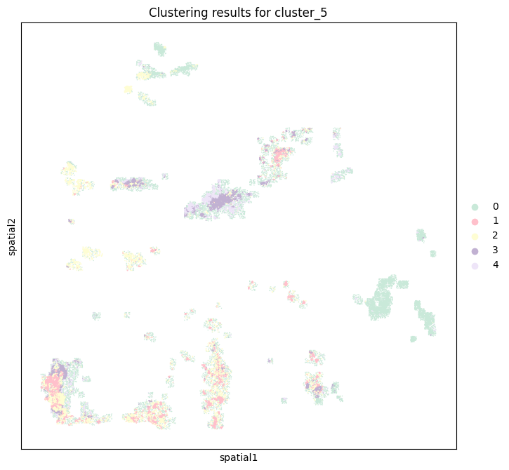
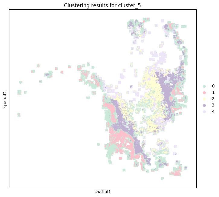
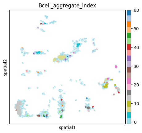
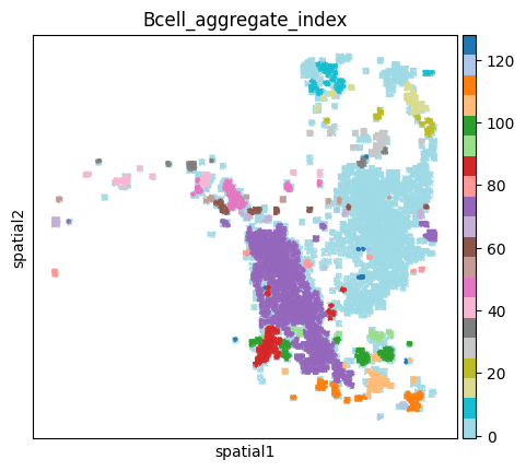
From the previous cell, 5 is the most appropriate number of clusters, so the number of categories is selected as 5, and the GMM model is used to cluster and the clustering results are visualized.

clusterer = B_HIT.st.tl.Cluster(n_clusters=5)  # 设置 5 个聚类
samples = set(enrichedAd.obs['sample'])
for sample in samples:
    print(sample)
    adata_tmp = enrichedAd[enrichedAd.obs['sample'].isin([sample])]
    clusterer.fit(adata_tmp, use_rep="X_cellcharter")
    clusterer.predict(adata_tmp, use_rep = 'X_scVI_hop3', store_labels = True, store_column = "cluster_5")
    B_HIT.st.pl.clustering_results(adata_tmp, cluster_column="cluster_5")

P0608_CC
P1121_LM